This GROMACS tutorial mostly follows the Protein-Ligand Complex Tutorial at GROMACS Tutorials by Justin A. Lemkul, Ph.D. with two important differences:
The workflow for setting up, running, and analysing a simulation consists of multiple and rather different steps. It is useful to perform these different steps in separate directories in order to avoid overwriting files or using wrong files.
For this tutorial the suggested directory layout is the following:
          - charmm36-mar2019/
          1. coord/
          2. protein/
          3. ligand/
          4. top/
          5. solvation/
          6. emin/
          7. posres/
          8. equilibration1
          9. equilibration2
          10. production/
          11. analysis/
The following is a short description of the directories:
The workflow for this exercise is such that each step is carried out in order and inside the appropriate directory. Each subdirectory depends on a specific task that is to be carried out, and is worked through in sequence. If a required file is needed in a subdirectory for use with the GROMACS command, copy that file to the subdirectory first.
The problem with a protein-ligand system is that the force field parameters, as well as other parameters, must be determined for both the protein and the small organic molecule that is within the protein. Parameters for the protein component are well-known and usually do not present any difficulty, but parameters for the small organic molecule must be obtained from a different force field. The following steps provide one way to obtain parameters for the small molecule organic ligand when the CHARMM force field is used.
Separate the original pdb file into two pdb files, one for the protein and one for the small-molecule ligand, jz4.
protein.pdb
jz4.pdb
gmx pdb2gmx -f protein.pdb -ff charmm36-mar2019 -water tip3p -ignh -o conf.pdb -nochargegrp
babel -i pdb jz4.pdb -o mol2 jz4.mol2
The jz4.mol2 is then submitted to the CGenFF server.`
Subsequently, the file jz4.str is now available for download, and can be used for both CHARMM and GROMACS.
A separate python file, cgenff_charmm2gmx_py2.py, is required for converting a the CHARMM jz4.str file into GROMACS input files.
The command:
cgenff_charmm2gmx_py2.py jz4 jz4.mol2 jz4.str charmm36-mar2019.ff
yields four files:
    jz4.itp - GROMACS topology file
    jz4.prm - GROMACS parameter file
    jz4_ini.pdb - PDB file for the initial coordinates of the jz4 ligand
    jz4.top
Three of the files, jz4.itp, jz4.prm, and jz4_ini.pdb are required GROMACS files for the ligand component of the protein-ligand complex.
The file, jz4.top, is a GROMACS prototype topology file which indicates where to place specific files for the protein and jz4 ligand. It is not used in this simulation,
and should not be confused with the required topol.top file, the system topolgy file.
gmx editconf -f protein.pdb -o boxed.pdb -c -d 1.0 -bt dodecahedron
gmx solvate -cs -cp boxed.pdb -o solvated.pdb -p topol.top
The system is now solvated but contains a charged protein. The output of pdb2gmx told us that the protein has a net charge of +6e
(based on its amino acid composition). If you missed this information in the pdb2gmx output, look at the last line of your [ atoms ]
directive in topol.top which should read (in part) "qtot 6." It is necessary to add ions to obtain a neutral system in order to perform Molecular Dynamics
with particle mesh ewald, for calculation of long-range electrostatic interactions.
Use grompp to assemble a .tpr file, using any .mdp file, for example, em.mdp.
gmx grompp -f em.mdp -c solvated.pdb -p topol.top -o ions.tpr
The ions.tpr files is then passed to genion:
gmx genion -s ions.tpr -o solvated_ions.pdb -p topol.top -pname NA -nname CL -conc 0.1
The specified atom names of ions are always the elemental symbol in all capital letters, along with the [ moleculetype ].
Residue names may or may not append the sign of the charge (+/-). Refer to ions.itp for proper nomenclature if you encounter difficulties.
The
[ molecules ]
; Compound        #mols
Protein_chain_A     1
JZ4                 1
SOL             13322
NA                 26
CL                 32
Now that the system is assembled, create the binary input using grompp and em.mdp as the input parameter file:
gmx grompp -f em.mdp -c solvated_ions.pdb -p topol.top -o em.tpr
Note that in the em.mdp file, the command: energygrps = Protein JZ4 is set, since it may be of interest later to examine the various components of the nonbonded interactions between your protein and ligand. This is a good practice in case anything goes wrong.
Make sure the topol.top file is updated each time when running genbox and solvate, or else you will get lots of nasty error messages ("number of coordinates in coordinate file does not match topology," etc).
We are now ready to invoke mdrun to carry out minimization:
gmx mdrun -v -deffnm em
The system should converge relatively quickly:
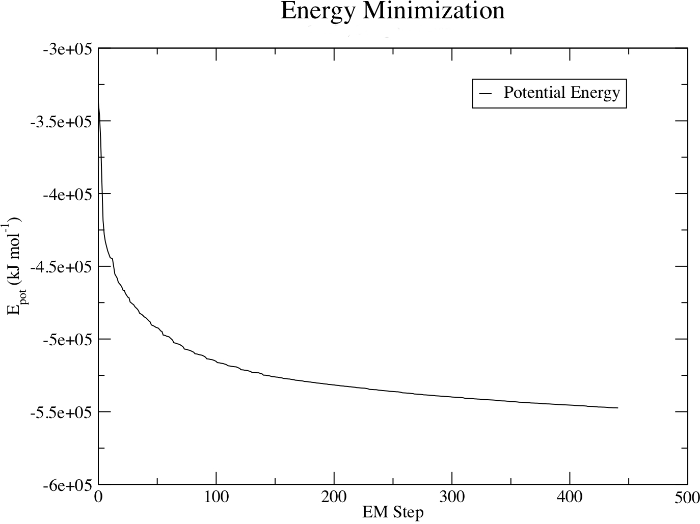
Steepest Descents converged to Fmax < 1000 in 178 steps
Potential Energy  = -5.0933919e+05
Maximum force     =  9.1495343e+02 on atom 1266
Norm of force     =  5.1248310e+01
It is possible to monitor various components of the potential energy using the energy module. The em.edr file contains all of the energy terms that GROMACS collects during energy minimization, and any .edr file can be analyzed using the GROMACS energy module:
gmx energy -f em.edr -o potential.xvg
At the prompt, type "10 0" to select Potential (10); zero (0) terminates input. You will be shown the average of Epot, and a file called "potential.xvg" will be written. To plot this data, use the Xmgrace plotting tool. The resulting plot should look something like this, demonstrating the nice, steady convergence of Epot:
Now that the system is at an energy minimum where bad contacts between atoms have been reduced, it is now possible to begin dynamics.
Equilibrating our protein-ligand complex will be much like equilibrating any other system containing a protein in water. However, there are a few special considerations, in this case:
Applying restraints to the ligand
Treatment of temperature coupling groups
The CGenFF server did not generate a separate restraint file for the ligand, analogous to the posre.itp for the protein, but GROMACS provides the means to do so with the genrestr module. Run the genrestr command on the jz4_ini.pdb file that we obtained from CGenFF:
gmx genrestr -f jz4_ini.pdb -o posre_jz4.itp -fc 1000 1000 1000
Now, this information must be included in the topology and can be performed in several ways. If we simply want to restrain the ligand whenever the protein is also restrained, add the following lines to the topology in the location indicated:
; Include Position restraint file
#ifdef POSRES
#include "posre.itp"
#endif

; Include ligand topology
#include "jz4.itp"

; Ligand position restraints
#ifdef POSRES
#include "posre_jz4.itp"
#endif

; Include water topology
#include "charmm36-mar2019/tip3p.itp"
Location matters! The line for posre_jz4.itp must be inserted in the topology after jz4.itp as indicated above.
The parameters within jz4.itp define a [ moleculetype ] directive for the ligand which end with the next {moleculetype] directive supplied by the
inclusion of the water topology file, tip3p.itp.
Placing the position of posre_jz4.itp anywhere else in the topology file will apply the position restraint parameters to the wrong moleculetype.
If a bit more control during equilibration is desired, i.e. restraining the protein and ligand independently, the inclusion of the ligand position restraint file in a different #ifdef block could be included in the following manner:
; Include Position restraint file
#ifdef POSRES
#include "posre.itp"
#endif

; Include ligand topology
#include "jz4.itp"

; Ligand position restraints
#ifdef POSRES_LIG
#include "posre_jz4.itp"
#endif

; Include water topology
#include "charmm36-mar2019/tip3p.itp"
In order to restrain both the protein and the ligand simultaneously, the command define = -DPOSRES -DPOSRES_LIG would have to be specificed in the nvt.mdp file.
There are many ways to specify the system under consideration, and these examples are meant only to illustrate the flexibility GROMACS provides. For a standard equilibration procedure, restraining the protein and ligand simultaneously is probably sufficient. Your own needs may vary.
Proper control of temperature coupling is a sensitive issue. Coupling every moleculetype to its own thermostat group is a bad idea. For the following command:
tc_grps = Protein JZ4 SOL CL
the system will probably blow up, since the temperature coupling algorithms are not stable enough to control the fluctuations in kinetic energy that groups with a few atoms (i.e., JZ4 and CL) will produce. Do not couple every single species in your system separately.
The typical approach is to set tc_grps =
Protein Non-Protein and carry on. Unfortunately, the
"Non-Protein" group also encompasses JZ4. Since JZ4 and the
protein are physically linked very tightly, it is best to consider
them as one single entity.
That is, JZ4 becomes part of the protein, for the purposes of temperature coupling. In the same way, the few Cl- ions we inserted become part of the solvent. To do this, a special index group is needed that merges the protein and JZ4. This is accomplished with the make_ndx module, supplying any coordinate file of the complete system. In this case, em.gro is used, the output for the minimized structure of the system:
gmx make_ndx -f em.gro -o index.ndx
...
  0 System              : 33037 atoms
  1 Protein             :  1693 atoms
  2 Protein-H           :  1301 atoms
  3 C-alpha             :   163 atoms
  4 Backbone            :   489 atoms
  5 MainChain           :   653 atoms
  6 MainChain+Cb        :   805 atoms
  7 MainChain+H         :   815 atoms
  8 SideChain           :   878 atoms
  9 SideChain-H         :   648 atoms
 10 Prot-Masses         :  1693 atoms
 11 non-Protein         : 31344 atoms
 12 Other               :    15 atoms
 13 JZ4                 :    15 atoms
 14 CL                  :     6 atoms
 15 Water               : 31323 atoms
 16 SOL                 : 31323 atoms
 17 non-Water           :  1714 atoms
 18 Ion                 :     6 atoms
 19 JZ4                 :    15 atoms
 20 CL                  :     6 atoms
 21 Water_and_ions      : 31329 atoms
Merge the "Protein" and "JZ4" groups with the following, where ">" indicates the make_ndx prompt:
> 1 | 13
> q
The command, tc_grps = Protein_JZ4 Water_and_ions, can be set to achieve the desired "Protein Non-Protein" effect.
Proceed with NVT equilibration using the nvt.mdp file:gmx grompp -f nvt.mdp -c em.gro -p topol.top -n index.ndx -o nvt.tpr gmx mdrun -deffnm nvt
A full explanation of the parameters used can be found in the GROMACS manual, in addition to the comments provided. Take note of a few parameters in the .mdp file:
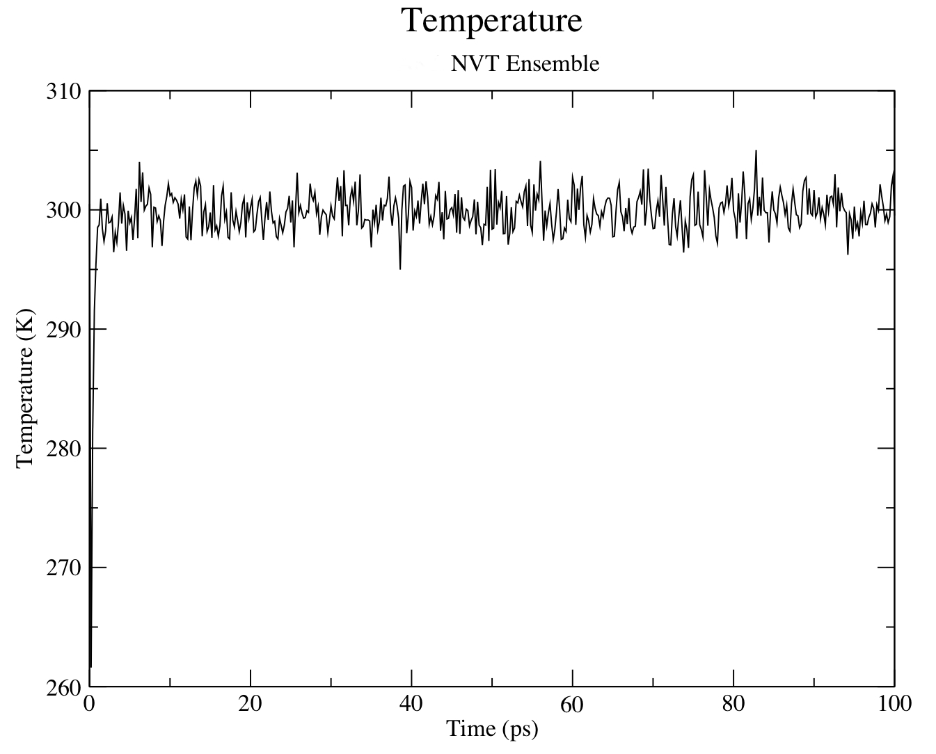
gmx energy -f nvt.edr
Type "15 0" at the prompt to select the temperature of the system and exit. The resulting plot should look something like the following:
Now that the NVT simulation is complete, one can proceed to an NPT simulation with the npt.mdp file:
The previous step, NVT equilibration, stabilized the temperature of the system. Prior to data collection, we must also stabilize the pressure (and thus also the density) of the system. Equilibration of pressure is conducted under an NPT ensemble, wherein the Number of particles(N), Pressure(P), and Temperature(T) are all constant. The ensemble is also called the "isothermal-isobaric" ensemble, and most closely resembles experimental conditions.
grompp and mdrun are used just as in the NVT equilibration. Note that we are now including the -t flag to include the checkpoint file from the NVT equilibration; This file contains all the necessary state variables to continue th simulation. To conserve the velocities produced during NVT, this file must be included. The coordinate file (-c) is the final output of the NVT equilibration.
The npt.mdp file used for an NPT equilibration is not drastically different from the parameter file used for NVT equilibration. Note the addition of the pressure coupling section, using the Parrinello-Rahman barostat.
Other changes inlude:
continuation = yes: continue the simulation from the NVT equilibration phase
gen_vel = no: velocities are read from the trajectory (see below)
gmx grompp -f npt.mdp -c nvt.gro -t nvt.cpt -p topol.top -n index.ndx -o npt.tpr

gmx mdrun -deffnm npt
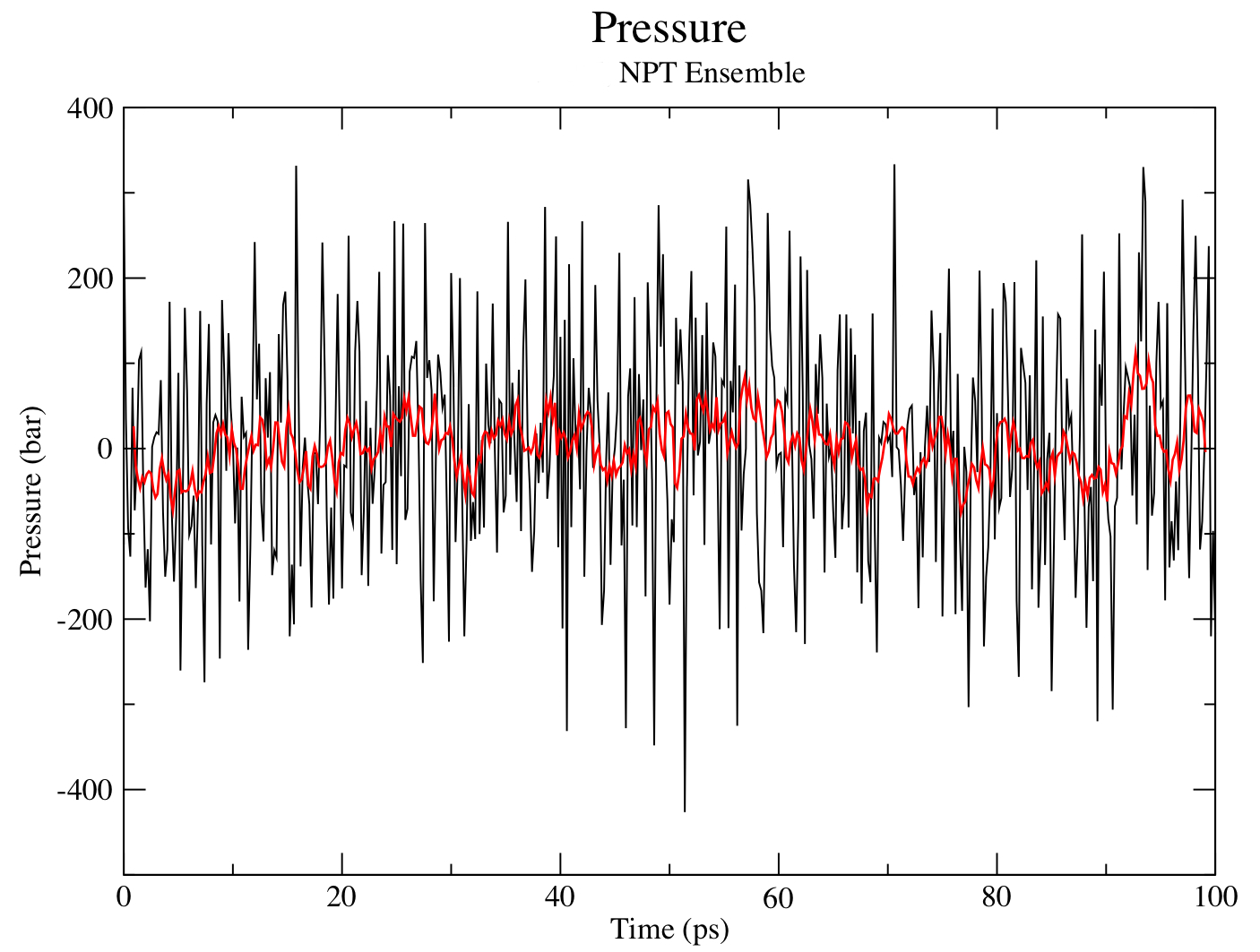
The pressure progression can be analyzed again using energy:
gmx energy -f npt.edr -o pressure.xvg
Type "16 0" at the prompt to select the pressure of the system and exit. The resulting plot should look something like the following:
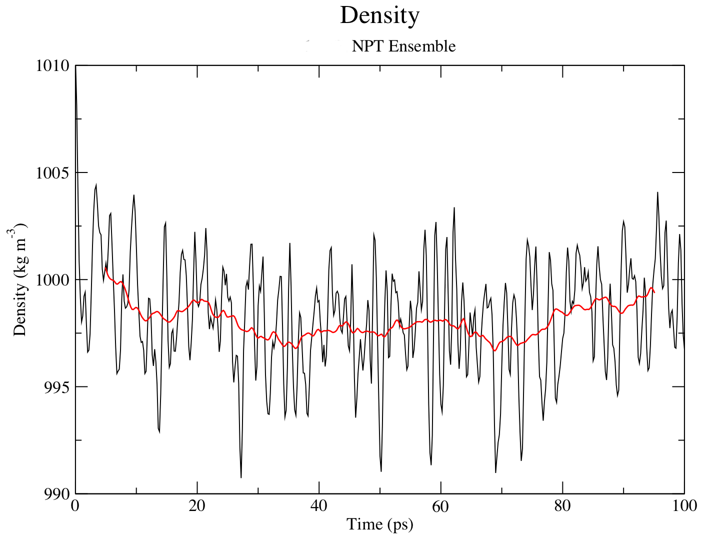
Let's take a look at density as well, this time using energy and entering "22 0" at the prompt.
gmx energy -f npt.edr -o density.xvg
Upon completion of the two equilibration phases, the system is now well-equilibrated at the desired temperature and pressure. We are now ready to release the position restraints and run production MD for data collection. The process will make use of the checkpoint file, which, in this case, now contains preserve pressure coupling information to grompp.
A 1-ns MD simulation will be run, the commands for which can be found in the md.mdp script file.
gmx grompp -f md.mdp -c npt.gro -t npt.cpt -p topol.top -n index.ndx -o md_0_1.tpr
trjconv is used as a post-processing tool to strip out coordinates, correct for periodicity, or manually alter the trajectory (time units, frame frequency, etc). trjconv can be used account for any periodicity in the system. The protein will diffuse through the unit cell, and may appear to "jump" across to the other side of the box. To account for such actions, issue the following:
gmx trjconv -s md_0_1.tpr -f md_0_1.xtc -o md_0_1_noPBC.xtc -pbc mol -ur compact
Select 0 ("System") for output. All analyses will be conducted on this "corrected" trajectory.
It is important to remember that GROMACS always works internally with an equivalent triclinic unit cell. To verify that the solvated molecule appears correctly in the octahedral simulation cell, it is necessary to transform the coordinates using the command:
gmx trjconv -s topol.tpr -f solvated_ions.pdb -o compact.pdb -ur compact -pbc mol
The types of data that are important for a simulation is a question to ask before running the simulation, so it is necessary to have ideas about the types of data you will want to collect. For this tutorial, a few basic tools will be introduced.
For a ligand like JZ4, hydrogen bonding is possible, so you might use gmx hbond to determine if any occurred.
gmx hbond -f npt.trr -s npt.tpr -num hbond.xvg
Is hydrogen bonding important?
The use of energygrps in the md.mdp file will allow an examination of the various components of the nonbonded potential between JZ4 and the protein.
gmx energy -f md.edr -o vdw.xvg

gmx energy -f md.edr -o  es.xvg
Do electrostatic interactions or van der Waals (hydrophobic) interactions dominate the association between these two species?
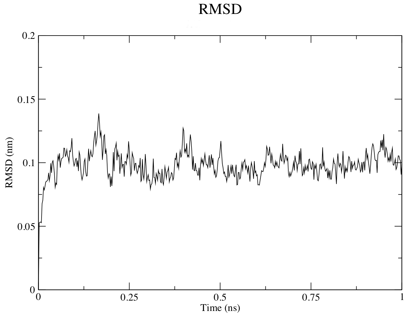
To look at structural stability, GROMACS has a built-in utility for RMSD calculations called rms. To use rms, issue this command:
gmx rms -s md_0_1.tpr -f md_0_1_noPBC.xtc -o rmsd.xvg -tu ns
Choose 4 ("Backbone") for both the least squares fit and the group for RMSD calculation. The -tu flag will output the results in terms of ns, even though the trajectory was written in ps. This is done for clarity of the output (especially if you have a long simulation - 1e+05 ps does not look as nice as 100 ns). The output plot will show the RMSD relative to the structure present in the minimized, equilibrated system:
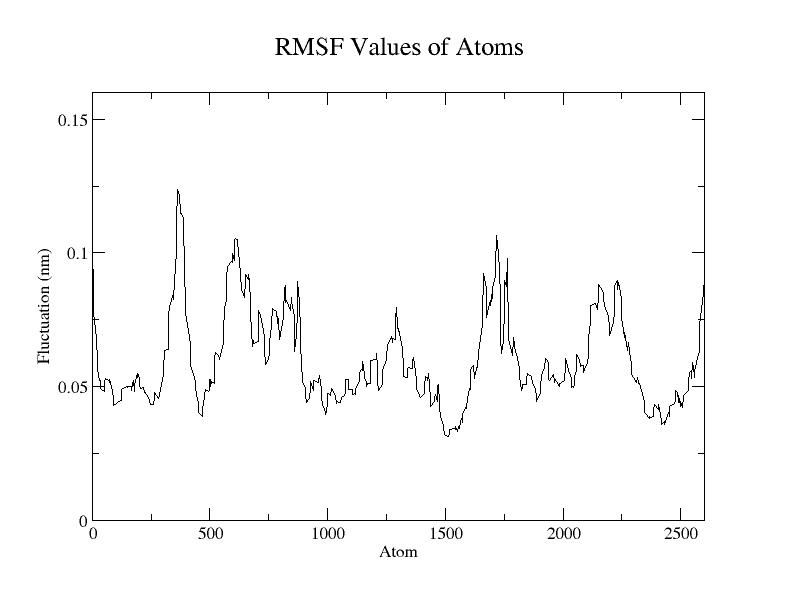
RMSF, the root mean square fluctuation, is a measurement similar to RMSD. Instead of indicating positional differences between entire structures over time, RMSF is a calculation of individual residue flexibility and provides information of how much a particular residue moves (fluctuates) during a simulation. RMSF per residue is typically plotted vs. residue number, and can indicate structurally which amino acids in a protein contribute the most to a molecular motion.
gmx rmsf -s md_0_1.tpr -f md_0_1_noPBC.xtc -o rmsf.xvg
For example, Choose Option 4 ("Backbone") for an RMSF calculation. The output plot will show the RMSF values or fluctuations for the atoms in each residue.
The radius of gyration of a protein is a measure of its compactness. If a protein is stably folded, it will likely maintain a relatively steady value of Rg. If a protein unfolds, its Rg will change over time. An analysis of the radius of gyration for protein-ligand simulation can be performed:
gmx gyrate -s md_0_1.tpr -f md_0_1_noPBC.xtc -o gyrate.xvg
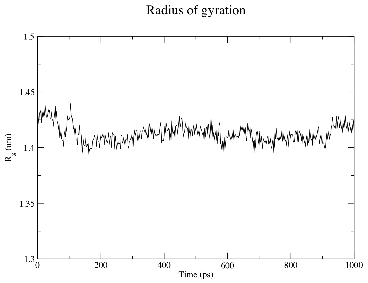
The figure above shows that the Rg is reasonably invariant, indicating that the protein remains very stable, in its compact (folded) form over the course of 1 ns at 300 K. This result is not unexpected, but illustrates an advanced capacity of GROMACS analysis that comes built-in.